function present_value(discount_rate, cashflows)
    v = 1.0
    pv = 0.0
    for cf in cashflows
        v = v / (1 + discount_rate)
        pv = pv + v * cf
    end
    return pv
end
present_value (generic function with 1 method)“Programs must be written for people to read, and only incidentally for machines to execute.” — Harold Abelson and Gerald Jay Sussman (Structure and Interpretation of Computer Programs, 1984)
Modern software engineering practices—version control, testing, documentation, and automated pipelines—make modeling more robust and reproducible. This chapter also covers data practices and workflow guidance.
In addition to the core concepts from computer science described so far, there are also neat ideas about the practice and experience of working with a code-based workflow that makes the end-to-end approach more powerful than the code itself.
It’s likely that the majority of a professional financial modeler’s time is often spent doing things other than building models, such as testing the model’s results, writing documentation, collaborating with others on the design, and figuring out how to share the model with others inside the company. This chapter covers how a code-first workflow makes each one of those responsibilities easier or more effective.
Financial models often face regulatory requirements around model validation, change management, and reproducibility. Software engineering practices directly support these requirements - version control provides a complete audit trail of all model changes, automated testing helps validate model behavior and demonstrates ongoing quality control, and comprehensive documentation meets regulatory demands for model transparency. For example, the European Central Bank’s Targeted Review of Internal Models (TRIM) Guide explicitly requires financial institutions to maintain documentation of model changes and validation procedures, which is naturally supported by Git commit history and continuous integration test reports that will be discussed in this chapter.
There are three essential topics covered in this chapter:
As the chapter progresses, some highly related topics are covered, bridging some of the conceptual ideas into practical implementations for your own code and models.
As a reminder, this chapter is heavily oriented to concepts that are applicable in any language, though the examples are illustrated using Julia for consistency and its clarity. The code examples would have direct analogues in other languages. In Chapter 21 many of these concepts will be reinforced and expanded upon with Julia-specific workflows and tips.
Testing is a crucial aspect of software engineering that ensures the reliability and correctness of code. In financial modeling, where accuracy is paramount, implementing robust testing practices is essential, and in many cases now often required by regulators or financial reporting authorities. It’s good practice regardless of requirements.
A test is implemented by writing a boolean expression after a @test macro:
@test model_output == desired_outputIf the expression evaluates to true, then the test passes. If the expression is anything else (false, or produces an error, or nothing, etc.) then the test will fail.
Here is an example of modeled behavior being tested. We have a function which will discount the given cashflows at a given annual effective interest rate. The cashflows are assumed to be equally spaced at the end of each period:
function present_value(discount_rate, cashflows)
v = 1.0
pv = 0.0
for cf in cashflows
v = v / (1 + discount_rate)
pv = pv + v * cf
end
return pv
endpresent_value (generic function with 1 method)We might test the implementation like so:
using Test

@test present_value(0.05, [10]) ≈ 10 / 1.05
@test present_value(0.05, [10, 20]) ≈ 10 / 1.05 + 20 / 1.05^2
Test Passed
The above test passes because the expression is true. However, the following will fail because we have defined the function assuming the given discount_rate is compounded once per period. This test will fail because the test target presumes a continuous compounding convention. A failing @test reports a test failure (showing actual vs expected). A stacktrace appears only if an error is thrown.
@test present_value(0.05, [10]) ≈ 10 * exp(-0.05 * 1)When testing results of floating point math, it’s a good idea to use the approximate comparison (≈, typed in a Julia editor by entering \approx<TAB>). Recall that floating point math is a discrete, computer representation of continuous real numbers. As perfect precision is not efficient, very small differences can arise depending on the specific numbers involved or the order in which the operations are applied.
In tests (as in the isapprox/≈ function), you can also further specify a relative tolerance and an absolute tolerance:
@test 1.02 ≈ 1.025 atol = 0.01
@test 1.02 ≈ 1.025 rtol = 0.005
Test Passed
The testing described in this section is sort of a ‘sampling’ based approach, wherein the modeler decides on some pre-determined set of outputs to test and determines the desired outcomes for that chosen set of inputs. That is, testing that 2 + 2 == 4 versus testing that a positive number plus a positive number will always equal another positive number. There are some more advanced techniques that cover the latter approach in Section 13.6.1.
More Julia-specific testing workflows are covered in Section 21.14.
Test Driven Development (TDD) is a software development approach where tests are written before the actual code. The process typically follows these steps:
TDD can be particularly useful in financial modeling as it helps clarify (1) intended behavior of the system and (2) how you think the system should work.
For example, if we want to create a new function which calculates an interpolated value between two numbers, we might first define the test like this:
# interpolate between two points (0,5) and (2,10)
@test interp_linear(0,2,5,10,1) ≈ (10-5)/(2-0) * (1-0) + 5
We’ve defined how it should work for a value inside the bounding \(x\) values, but writing the test has us wondering… should the function error if x is outside of the left and right \(x\) bounds? Or should the function extrapolate outside the observed interval? The answer to that depends on exactly how we want our system to work. Sometimes the point of such a scheme is to extrapolate, other times extrapolating beyond known values can be dangerous. For now, let’s say we would like to have the function extrapolate, so we can define our test targets to work like that:
@test interp_linear(0,2,5,10,-1) ≈ (10-5)/(2-0) * (-1 - 0) + 5
@test interp_linear(0,2,5,10,3) ≈ (10-5)/(2-0) * (3 - 0) + 5
By thinking through what the correct result for those different functions is, we have forced ourselves to think about how the function should work generically:
function interp_linear(x1,x2,y1,y2,x)
    # slope times difference from x1 + y1
    return (y2 - y1) / (x2 - x1) * (x - x1) + y1
end
interp_linear (generic function with 1 method)And we can see that our tests defined above would pass after writing the function.
@testset "Linear Interpolation" begin
    @test interp_linear(0,2,5,10,1) ≈ (10-5)/(2-0) * (1-0) + 5
    @test interp_linear(0,2,5,10,-1) ≈ (10-5)/(2-0) * (-1 - 0) + 5
    @test interp_linear(0,2,5,10,3) ≈ (10-5)/(2-0) * (3 - 0) + 5
end;
Test Summary: | Pass Total Time Linear Interpolation | 3 3 0.0s
Testing is great, but what if some things aren’t tested? For example, we might have a function that has a branching if/else condition and only ever tests one branch. Then when the other branch is encountered in practice it is more vulnerable to having bugs because its behavior was never double checked. Wouldn’t it be great to tell whether or not we have tested all of our code?
The good news is that there is! Test coverage is a measurement related to how much of the codebase is covered by at least one associated test case. In the following example, code coverage would flag that the ... other logic is not covered by tests and therefore encourage the developer to write tests covering that case:
function asset_value(strike,current_price)
    if current_price > strike
    # ... some logic
    else
    # ... other logic
    end
end

@test asset_value(10,11) ≈ 1.5
From the coverage statistics, it’s possible to determine a score for how well a given set of code is tested. 100% coverage means every line of code has at least one test that double checked its behavior.
Testing is only as good as the tests that are written. You could have 100% code coverage for a codebase with only a single rudimentary test covering each line. Or the test itself could be wrong! Testing is not a cure-all, but does encourage best practices.
Test coverage is also a great addition when making modification to code. It can be set up such that you receive reports on how the test coverage changes if you were to make a certain modification to a codebase. An example might look like this for a proposed change which added 13 lines of code, of which only 11 of those lines were tested (“hit”). The total coverage percent has therefore gone down (-0.49%) because the proportion of new lines covered by tests is \(11/13 = 84\%\), which is lower than the original coverage rate of 90%.
@@            Coverage Diff             @@
##         original    modif    +/-   ##
==========================================
- Coverage   90.00%   89.51%   -0.49%
==========================================
  Files           2        2
  Lines         130      143      +13
==========================================
+ Hits          117      128      +11
- Misses 13 15 +2 Different tests can emphasize different aspects of model behavior. You could be testing a small bit of logic, or test that the whole model runs if hooked up to a database. The variety of this kind of testing has given rise to various named types of testing, but it’s somewhat arbitrary and the boundaries between the types can be fuzzy. Common types include unit testing, integration testing, and regression testing.
| Test Type | Description |
|---|---|
| Unit Testing | Verifies the functionality of individual components or functions in isolation. It ensures that each unit of code works as expected. |
| Integration Testing | Checks if different modules or services work together correctly. It verifies the interaction between various components of the system. |
| End-to-End Testing | Simulates real user scenarios to test the entire application flow from start to finish. It ensures the system works as a whole. |
| Functional Testing | Validates that the software meets specified functional requirements and behaves as expected from a user’s perspective. |
| Regression Testing | Ensures that new changes or updates to the code haven’t broken existing functionality. It involves re-running previously completed tests. |
There are other types of testing that can be performed on a model, such as performance testing, security testing, acceptance testing, etc., but these types of tests are outside of the scope of what we would evaluate with an @test check. It is possible to create more advanced, mathematical-type checks and tests, which are introduced in Section 13.6.1.
Test reports and test coverage are a wonderful way to demonstrate regular and robust testing for compliance. It is important to read and understand any limitations related to testing in your choice of language and associated libraries.
The most important part of code for maintenance purposes is plainly written notes for humans, not the compiler. This includes in-line comments, docstrings, reference materials, and how-to pages, etc. Even as a single model developer, writing comments for your future self is critical for model maintenance and ongoing productivity.
Docstrings (documentation strings) are intended to be a user-facing reference and help text. In Julia, docstrings are just strings placed in front of definitions. Markdown1 is available (and encouraged) to add formatting within the docstring.
Here’s an example with some various features of documentation shown:
"""
1    calculate_bond_price(
    face_value,
    coupon_rate,
    years_to_maturity,
    market_rate
    )

Calculate the price of a bond using discounted cash flow method.

Parameters:
- `face_value`: The bond's par value
- `coupon_rate`: Annual coupon rate as a decimal
- `years_to_maturity`: Number of years until the bond matures
- `market_rate`: Current market interest rate as a decimal

Returns:
- The calculated bond price

2## Examples:

```julia-repl
julia> calculate_bond_price(1000, 0.05, 10, 0.06)
925.6126256977221
```

3## Extended help:

This function uses the following steps to calculate the bond price:
1. Convert annual rates to semi-annual rates
2. Calculate the present value of all future coupon payments
3. Calculate the present value of the face value at maturity
4. Sum these components to get the total bond price

The calculation assumes semi-annual coupon payments, which is standard in many markets.
"""
function calculate_bond_price(face_value, coupon_rate, years_to_maturity, market_rate)
    # ... function definition as above
endThe last point, the Extended help section is shown when using help mode in the REPL and including an extra ?. For example, in the REPL, typing ?calculate_bond_price will show the docstring up through the examples. Typing ??calculate_bond_price will show the docstring in its entirety.
Docstrings become even more valuable when you hook them into automated documentation generators such as Documenter.jl. Documenter ingests Markdown pages plus in-code docstrings, renders math, runs doctests, and publishes a searchable site every time CI runs. Writing rich docstrings up front means your docsite, help mode, and notebook snippets stay perfectly in sync.
Docsites, or documentation sites, are websites that are generated to host documentation related to a project. Modern tooling associated with programming projects can generate a really rich set of interactive documentation while the developer/modeler focuses on simple documentation artifacts.
Specifically, modern docsite tooling generally takes in markdown text pages along with the in-code docstrings and generates a multi-page site that has navigation and search.
Typical contents of a docsite include:
A Quickstart guide that introduces the project and provides an essential or common use case that the user can immediately run in their own environment. This conveys the scope and demonstrates intended usage.
Tutorials are typically worked examples that introduce basic aspects of a concept or package usage and work up to more complex use cases.
Developer documentation is intended to be read by those who are interested in understanding, contributing, or modifying the codebase.
Reference documentation describes concepts and available functionality. A subset of this is API, or Application Programming Interface, documentation which is the detailed specification of the available functionality of a package, often consisting largely of docstrings like the previous example.
Docsite generators are generally able to look at the codebase and from just the docstrings create a searchable, hierarchical page with all of the content from the docstrings in a project. This basic docsite feature is incredibly beneficial for current and potential users of a project.
To go beyond creating a searchable index of docstrings requires additional effort (time well invested!). Creating the other types of documentation (quick start, tutorials, etc.) is mechanically as simple as creating a new markdown file. The hard part is learning how to write quality documentation. Good technical writing is a skill developed over time - but at least the technical and workflow aspects have been made as easy as possible!
Version control systems (VCS) refer to the tracking of changes to a codebase in a verifiable and coordinated way across project contributors. VCS underpins many aspects of automating the mundane parts of a modeler’s job. Benefits of VCS include (either directly, or contribute significantly to):
These features are massively beneficial to a financial modeler! A lot of the overhead in a modeler’s job becomes much easier or automated through this tooling.
Among several competing options (CVS, Mercurial, Subversion, etc.), Git is the predominant choice as of this book’s writing and therefore we will focus on Git concepts and workflows.
This section will introduce Git related concepts at a level deeper than “here’s the five commands to run” but not at a reference-level of detail. The point of this is to reveal some of the underlying technology and approaches so that you can recognize where similar ideas appear in other areas and understand some of the limitations of the technology.
Git is free and open-source software that tracks changes in files using a series of snapshots. Git itself is the underlying software tool and is a command-line tool at its core. However, you will often interact with it through various interfaces (such as a graphical user interface in VS Code, GitKraken, or other tool).
Each snapshot, or commit, stores references to the files that have changed2. All of this is stored in a .git/ subfolder of a project, which is automatically created upon initializing a repository. This folder may be hidden by default by your filesystem. You generally never need to modify anything inside the .git/ folder yourself as Git handles this for you. Git tracks files in the repository working tree (the directory containing the .git folder and its subdirectories). It does not track directories outside the repository.
Think of Git as a series of ‘save points’ in a video game. Each time you reach a milestone, you create a ‘commit’ - a snapshot of your entire project. If you make a mistake later, you can always reload a previous save point. ‘Branches’ are like alternate timelines, allowing you to experiment with new features without affecting your main saved game.
Hashes indicate a verifiable snapshot of a codebase. For example, a full commit ID (a hash) 40f141303cec3d58879c493988b71c4e56d79b90 will always refer to a certain snapshot of the code, and if there is a mismatch in the git history between the contents of the repository and the commit’s hash, then the git repository is corrupted and it will not function. A corrupted repository usually doesn’t happen in practice, of course! You might see hashes shortened to the first several characters (e.g. 40f1413) and in the following examples we’ll shorten the hypothetical hashes to just three characters (e.g. 40f).
A codebase can be branched, meaning that two different versions of the same codebase can be tracked and switched between. Git lends itself to many different workflows, but a common one is to designate a primary branch (call it main) and make modifications in a new, separate branch. This allows for non-linear and controlled changes to occur without potentially tainting the main branch. It’s common practice to always have the main branch be a ‘working’ version of the code that can always ‘run’ for users, while branches contain works-in-progress or piecemeal changes that temporarily make the project unable to run.
The commit history forms a directed acyclic graph (DAG) representing the project’s history. That is, there is an order to the history: the second commit is dependent on the first commit. From the second commit, two child commits may be created that both have the second commit as their parent. Each one of these commits represents a stored snapshot of the project at the time of the commit.
A directory structure demonstrating where git data is stored and what content is tracked after initializing a repository in the tracked-project directory. Note how untracked-folder is not the parent directory of the .git directory so it does not get tracked by Git.
/home/username
├── untracked-folder
│   ├── random-file.txt
│   └── ...
└── tracked-project
    ├── .git
    │   ├── config
    │   ├── HEAD
    │   └── objects
    │       └── ...
    ├── .gitignore
    ├── README.md
    └── src
        ├── MainProject.jl
        ├── module1.jl
        └── module2.jl
Under the hood, the Git data stored inside the .git/ includes things such as binary blobs, trees, commits, and tags. Blobs store file contents, trees represent directories, commits point to trees and parent commits, and tags provide human-readable names for specific commits. This structure allows Git to efficiently handle branching, merging, and maintaining project history.
Table 12.1 shows an example workflow for trying to fix an erroneous function present_value which was written as part of a hypothetical FileXYZ.jl file. This example is trivial, but in a larger project where a ‘fix’ or ‘enhancement’ may span many files and take several days or weeks to implement, this type of workflow becomes like a superpower compared to traditional, manual version control approaches. It sure beats an approach where you end up with filenames like FileXYZ v23 July 2022 Final.jl!
pv) function. The branch name/commit ID shows which version you would see on your own computer/filesystem. The inactive branches are tracked in Git but do not manifest themselves on your filesystem unless you checkout that branch.
Branch main , FileXYZ.jl file |
Branch fix_function , FileXYZ.jl file |
Action | Active Branch (Abbreviated Commit ID) |
|---|---|---|---|
|
Does not yet exist | Write original function which forgets to take into account the time. Stage and commit it to the main branch.Git commands: git add FileXYZ.jl, then git commit -m 'add pv function' |
main( ...58b) |
| ” | |
Create a new branch fix_function.Git command: git branch fix_function |
main( ...58b) |
| ” | ” | Checkout the new branch and make it active for editing. The branch is different but is starting from the existing commit. Git command: git checkout fix_function |
fix_function( ...58b) |
| ” | |
Edit and save the changed file. No git actions taken. | fix_function( ...58b) |
| ” | ” | “Stage” the modified file, telling git that you are ready to record (“commit”) a new snapshot of the project. Git command: git add FileXYZ.jl |
fix_function( ...58b) |
| ” | ” | Commit a new snapshot of the project by committing with a note to collaborators saying fix: present value logicGit command: git commit -m 'fix: present value logic' |
fix_function( ...6ac) |
| ” | ” | Switch back to the primary branch Git command: git checkout main |
main( ...58b) |
|
” | Merge changes from other branch into the main branch, incorporating the corrected version of the code.Git command: git merge fix_function |
main( ...b90) |
A visual representation of the git repository and commits for the actions described in Table 12.1 might be as follows, where the ...XXX is the shortened version of the hash associated with that commit.
main branch         :  ...58b       →   ...b90
                          ↓           ↗
fix_function branch :  ...58b → ...6ac
The “staging” aspect will be explained next.
Most teams wrap the branch workflow inside a pull-request (PR) or merge-request process. A typical cadence for an actuarial change is:
fix: correct PV logic for monthly products) and a link to the model-change ticket or associated GitHub Issue number.Writing clear commit messages (e.g., Conventional Commits) and using PR templates that ask for “risk assessment” or “validation evidence” makes it easy to satisfy SOX/CECL/Solvency documentation requirements without a separate Word document.
Staging (sometimes called the “staging area” or “index”) is an intermediate step between making changes to files and recording those changes in a commit. Think of staging as preparing a snapshot - you’re choosing which modified files (or even which specific changes within files) should be included in your next commit. When you modify files in your Git repository, those changes are initially “unstaged.” Using the git add command (or your Git GUI’s staging interface) moves changes into the staging area. This two-step process - staging followed by committing - gives you precise control over which changes get recorded together. Here’s a typical workflow:
This is particularly useful when you’re working on multiple features or fixes simultaneously. For example, imagine you’re updating a financial model and you:
You could stage and commit the bug fix and documentation separately, keeping the work-in-progress feature changes unstaged until they’re complete. This creates a cleaner, more logical project history where each commit represents one coherent change.
Think of staging as preparing a shipment: you first gather and organize the items (staging), then seal and send the package (committing). This extra step helps maintain a well-organized project history where each commit represents a logical, self-contained change.
Git is traditionally a command-line based tool, however we will not focus on the command line usage as more beginner friendly and intuitive interfaces are available from different available software. The branching and nodes are well suited to be represented visually.
Some recommend Git tools with a graphical user interface (GUI):
Github Desktop interfaces nicely with Github and provides a GUI for common operations.
Visual Studio Code has an integrated Git pane, providing a powerful GUI for common operations.
GitKraken is free for open source repositories but requires payment for usage in enterprise or private repository environments. GitKraken provides intuitive interfaces for handling more advanced operations, conflicts, or issues that might arise when using Git.
Git is a distributed VCS, meaning that copies of the repository and all its history and content can live in multiple locations, such as on two colleagues’ computer as well as a server. In this distributed model, what happens if you make a change locally?
Git maintains a local repository on each user’s machine, containing the full project history. This local repository includes the working directory (current state of files), staging area (changes prepared for commit), and the .git directory (metadata and object database). When collaborating, users push and pull changes to and from remote repositories. Git uses a branching model, allowing multiple lines of development to coexist and merge when ready.
The primary branch of a project is typically named the main branch. This change reflects a shift from the older master branch name, which some projects may still use.
Layered onto core Git functionality, services like Github provide interfaces which enhance the utility of VCS. A major example of this is Pull Requests (or PRs), which are a process of merging Git branches in a way that allows for additional automation and governance.
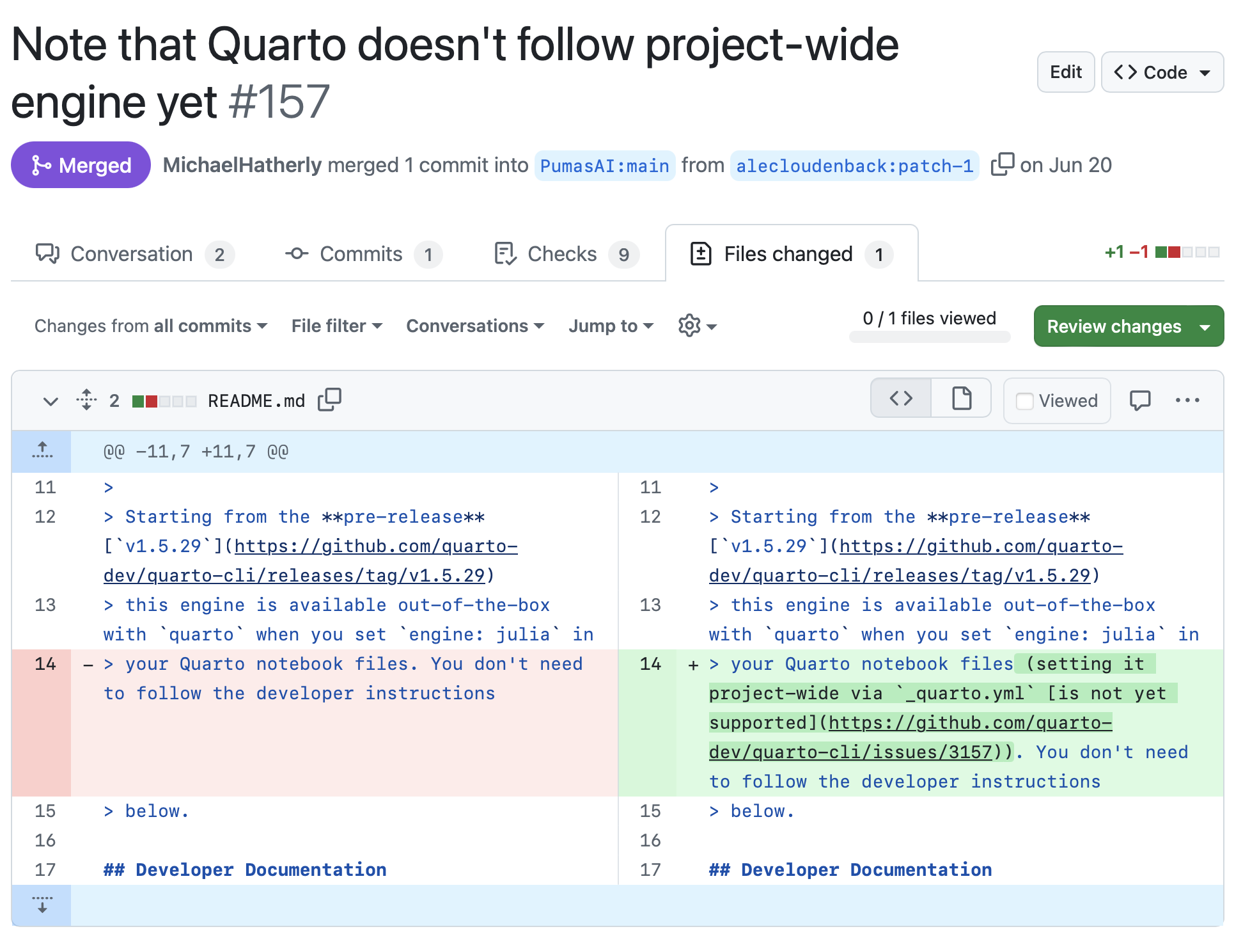
The following is an example of a PR on a repository adding a small bit of documentation to help future users. We’ll walk through several elements to describe what’s going on:
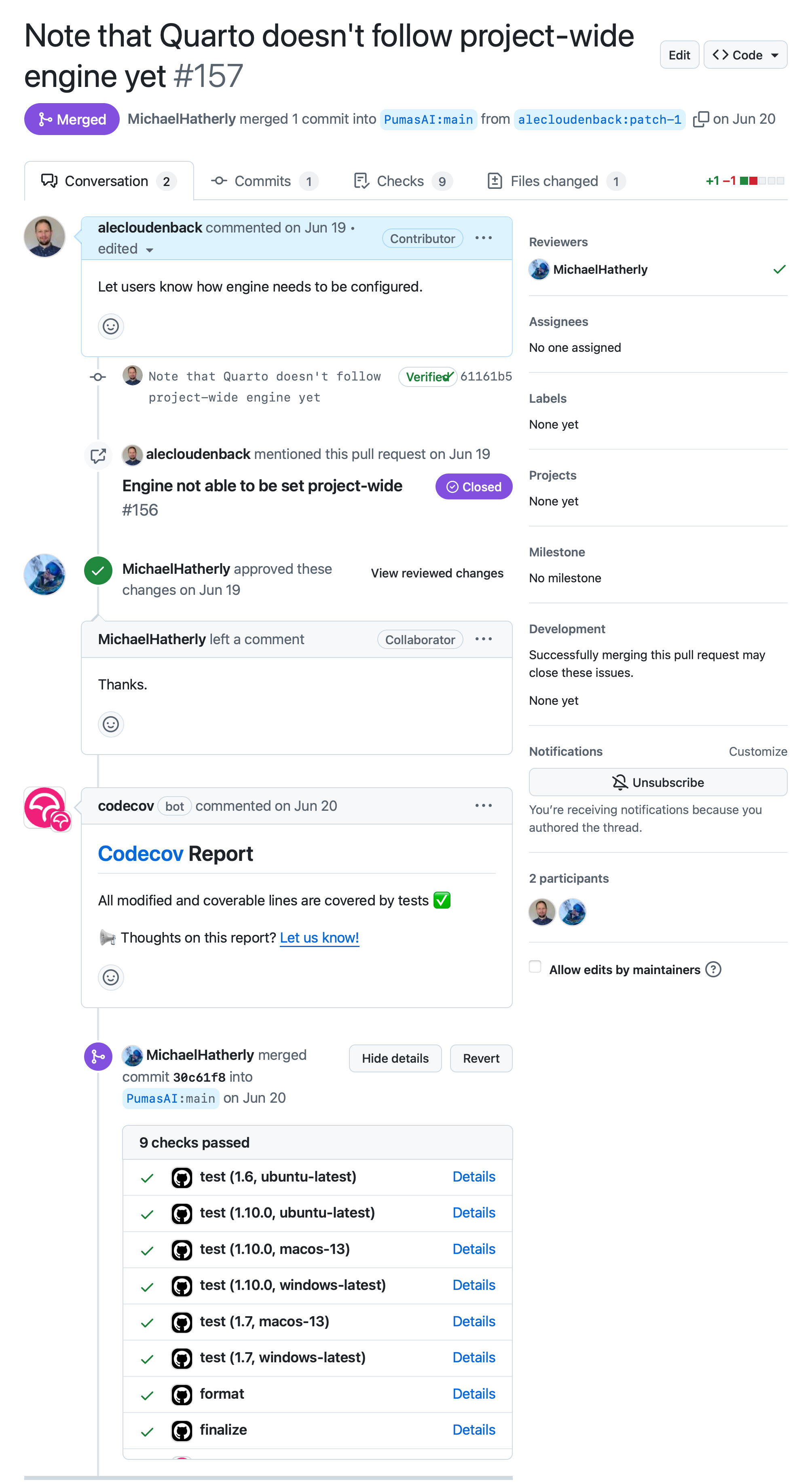
Referencing Figure 12.1, several elements are worth highlighting. In this pull request the author of this change, alecloudenback, is proposing to modify the QuartoNotebookRunner repository, which is not a repository for which the user alecloudenback has any direct rights to modify. After having made a copy of the repository (a “fork”), creating a new branch, making modifications, and committing those changes… a pull request has been made to modify the primary repository.
+1 -1 ■■□□□ is an indication of what’s changed. In this case, a single line of code (documentation, really) was removed (-1) and replaced with another (+1)MichaelHatherly) is a collaborator with rights to modify the destination repository and has been assigned to review this change before merging it into the main branch.The features described here can take modelers many hours of time - testing, review of changes, sign-off tracking, etc. In this Git-based workflow, the workflow above happens frictionlessly and much of it is automated. This is such a powerful paradigm that should be adopted within the financial industry and especially amongst modelers.
CI pipelines turn “remember to rerun the model” into code. A minimal Julia CI workflow usually runs:
julia --project -e 'using Pkg; Pkg.instantiate(); Pkg.test()'docs/make.jl) and style checks (using JuliaFormatter; format(".")).Because GitHub Actions, GitLab CI, and Azure Pipelines capture logs and artifacts automatically, each pull request carries a timestamped record of which Julia version, OS, and dependency set produced the numbers. Regulators can accept these logs as part of model change evidence because they are immutable and repeatable.
Git alone is not well suited for large, frequently changing binary files. Instead, the approach is to combine git with a data version control tool. These tools essentially replace the data (often called binary data or a blob) with a content hash in the git snapshots. The actual content referred to by the hash is then located elsewhere (e.g. a hosted server).
Content hashes are the output of a function that transforms arbitrary data into a string of data. Hashes are very common in cryptography and in areas where security/certainty is important. Eliding the details of how they work exactly, what’s important to understand for our purposes is that a content hash function will take arbitrary bits and output the same set of data each time the function is called on the original bits.
For example, it might look something like this:
using SHA

data = "A data file contents 123"
bytes2hex(sha256(codeunits(data)))"b37600bffd200c98b9bb9f8deef14e1612851fa2ff5e22f24bff870423607c66"If it’s run again on the same inputs, you get the same output:
# Same input → same hash
bytes2hex(sha256(codeunits(data)))"b37600bffd200c98b9bb9f8deef14e1612851fa2ff5e22f24bff870423607c66"And if the data is changed even slightly, then the output is markedly different:
# Slight change → very different hash
data2 = "A data file contents 124"
bytes2hex(sha256(codeunits(data2)))"773c90b32c6a8b927d5f7e422e2bd5240db587edcaa9cf6b753273b097782080"Use a cryptographic hash (e.g., SHA-256) to derive a stable, deterministic content hash. Base.hash is intentionally randomized for security and is not suitable for content-addressed storage.
This is used in content-addressed systems like Data Version Control (Section 12.5.4) and Artifacts (Section 12.6.3) to ask for, and confirm the accuracy of, data instead of trying to address the data by its location. That is, instead of trying to ask to get data from a given URL (e.g. http://adatasource.com/data.csv) you can set up a system which keeps track of available locations for the data that matches the content hash. Something like (in Julia-ish pseudocode):
storage_locations = Dict(
    "0x4d7e8e449afd1c48" => [
        "http://datasets.com/1231234",
        "http://companyintranet.com/admin.csv",
        "C:/Users/your_name/Documents/Data/admin.csv"
    ]
)

function get_data(hash,locations)
    for location in locations[hash]
        if is_available(location)
            return get(location)
        end
    end

    # if loop didn't return data
    return nothing
endOnce you have created a package, the next best feeling after having it working is having someone else also use the tool. Julia has a robust way to distribute and manage dependencies. This section will cover essential and related topics to distributing your project publicly or with an internal team.
Registries are a way to keep track of packages that are available to install, which is more complex than it might seem at first. The registry needs to keep track of:
The Julia General Registry (“General”) is the default registry that comes loaded when installing Julia. From a capability standpoint, there’s nothing that separates General from other registries, including ones that you can create yourself. At its core, a registry can be seen as a Git repository where each new commit just adds information associated with the newly registered package or version of a package.
For distributing packages in a private, or smaller public group see Section 23.9.2.1.
At its core, General is essentially the same as a local registry described in the prior section. However, there’s some additional infrastructure supporting General. Registered packages get backed up, cached for speed, and multiple servers across the globe are set up to respond to Pkg requests for redundancy and latency. Nothing would stop you from doing the same for your own hosted registry if it got popular enough!
A local registry is a great way to set up internal sharing of packages within an organization. Services do exist for “managed” package sharing, adding enterprise features like whitelisted dependencies, documentation hosting, a ‘hub’ of searchable packages.
Versioning is an important part of managing a complex web of dependencies. Versioning is used to let both users and the computer (e.g. Pkg) understand which bits of code are compatible with others. For this, consider your model/program’s Application Programming Interface (API). The API is essentially defined by the outputs produced by your code given the same inputs. If the same inputs are provided, then for the same API version the same output should be provided. However, this isn’t the only thing that matters. Another is the documentation associated with the functionality. If the documentation said that a function would work a certain way, then your program should follow that (or fix the documentation)!
Another case to consider is what if new functionality was added? Old code need not have changed, but if there’s new functionality, how to communicate that as an API change? This is where Semantic Versioning (SemVer) comes in: semantic means that your version of something is intended to convey some sort of meaning over and above simply incrementing from v1 to v2 to v3, etc.
Semantic Versioning (SemVer) is one of the most popular approaches to software versioning. It’s not perfect but has emerged as one of the most practical ways since it gets a lot about version numbering right. Here’s how SemVer is defined3:
Given a version number MAJOR.MINOR.PATCH, increment the:

- MAJOR version when you make incompatible API changes
- MINOR version when you add functionality in a backward compatible manner
- PATCH version when you make backward compatible bug fixes
So here are some examples of SemVer, if our package’s functionality for v1.0.0 is like this:
""" my_add(x,y)

Add the numbers x and y together
"""
my_add(x,y) = x - y
Patch change (v1.0.1): Fix the bug in the implementation:
""" my_add(x,y)
Add the numbers x and y together
"""
my_add(x,y) = x + y
This is a patch change because it fixes a bug without changing the API. The function still takes two arguments and returns their sum, as originally documented.
Minor change (v1.1.0): Add new functionality in a backward-compatible manner:
""" my_add(x,y)
Add the numbers x and y together

my_add(x,y,z)
Add the numbers x, y, and z together
"""
my_add(x,y) = x + y
my_add(x,y,z) = x + y + z
This is a minor change because it adds new functionality (the ability to add three numbers) while maintaining backward compatibility with the existing two-argument version.
Major change (v2.0.0): Make incompatible API changes:
""" add_numbers(numbers...)
Add any number of input arguments together. This
function replaces `my_add` from prior versions.
"""
add_numbers(numbers...) = sum(numbers)
This is a major change because it fundamentally alters the API. The function name has changed, and it now accepts any number of arguments instead of specifically two or three. This change is not backward compatible with code using the previous versions, so a major version increment is necessary.
Numbers need not roll over to the next digit when they hit 10. That is, it’s perfectly valid to go from v1.09.0 to v1.10.0 in SemVer.
Sometimes you’ll see a package with a version that starts with zero, such as v0.23.1. We recommend that as soon as you register a package, to make it a v1. v1 need not indicate the package is “complete” (what software is?), so don’t hold back on calling it v1. You’re letting users install it easily, so you might as well call it the first version and move on!
According to SemVer’s rules:
Major version zero (0.y.z) is for initial development. Anything MAY change at any time. The public API SHOULD NOT be considered stable.
Most packages put an upper bound on compatibility so that major or minor changes in upstream packages are less likely to cause issues in their own packages. This can be somewhat painful to depend on a package which has a major version 0 (i.e. v0.x.x). You have to assume minor version bumps are backward incompatible changes, but the author might intend it to be a feature release. You should have skepticism of just upgrading to the new version of the dependency. It takes work on the downstream dependencies to decide if they should upgrade, adding mental and time loads to other authors and users.
This is why once you have anyone else depending on the package, going straight to v1 is helpful because you have finer-grained control over the release versioning and the meaning behind each new version number.
Artifacts are a way to distribute content-addressed (Note 12.1) data and other dependencies. An example use case is if you want to distribute some demonstration datasets with a package. When a package is added or updated, the associated data is pulled and un-archived by Pkg instead of the author of the package needing to manually handle data dependencies. Aside from this convenience, it means that different packages could load the same data without duplicating the data download or storage (since the data is content-addressed). The use-case is not real-time data, as the content-hash can only be updated per package version.
For example, the MortalityTables.jl package redistributes various publicly available, industry mortality tables. Inside the repository, there’s an Artifacts.toml file specified like:
#| code-overflow: wrap
#/Artifacts.toml

["mort.soa.org"]
1git-tree-sha1 = "6164a6026f108fe95828b689fcd3b992acbff7c3"

    [["mort.soa.org".download]]
2    sha256 = "6f5eb4909564b55a3397ccf4f4c74290e002f7e2e2474cebeb224bb23a9a2606"
url = "https://github.com/JuliaActuary/Artifacts/raw/v2020-02-15/mort.soa.org/2020-02-15.tar.gz"Then, within the package the data artifact can be referenced and handled by the artifact system rather than needing to manually handle it. That is, the data is reference-able like this:
using Pkg.Artifacts
1table_dir = artifact"mort.soa.org"md"..." is another example, specifying that the content of the string is Markdown content.
As opposed to something like this:
# pseudo Julia code
table_dir = if is_first_package_run

    data_path = download("url_of_data.tar.gz") # download to a temp location
    mv(data_path, "/somewhere/to/keep/data.tar.gz") # move to a 'permanent' location
    extract("/somewhere/to/keep/data.tar.gz") # extract contents
    "/somewhere/to/keep/data/" # return data path
else
    "/somewhere/to/keep/data/" # return pre-processed path

endUtility Packages such as ArtifactUtils.jl can assist in creating correct entries for Artifacts.toml files.
Artifacts support .tar (uncompressed) and .tar.gz because that compression format enjoys more universal support and features than the .zip format most common on Windows systems.
A well-structured Julia package demonstrates key software engineering principles in action. The JuliaTemplateRepo repository demonstrates best practices for:
This open-source template serves as a reference implementation.
The PkgTemplates.jl package will allow you to create an empty repository with all of the testing, documentation, Git, and continuous integration scaffolding already in place.
Markdown is a type of plain text which can be styled for better communication and aesthetics. E.g. **some text** would render as boldface: some text. This book was written in Markdown and all of the styling arose as a result of plain text files written with certain key elements.↩︎
Git uses a content-addressable filesystem, meaning it stores data as key-value pairs. The key is a hash of the content, ensuring data integrity and allowing efficient storage of identical content. For more on hashes, see the Content Hashes callout later in this chapter.↩︎
You can read more at SemVer.org.↩︎
12.4.1 Comments
Comments are meant for the developer to aid in understanding a certain bit of code. A bit of time-tested wisdom is that after several weeks, months, or years away from a piece of code, something that seemed ‘obvious’ at the time tends to become perplexing at a later time. Writing comments is as much for yourself as it is your colleagues or successors. Focus comments on why something is done (business constraints, regulatory rules, data quirks) rather than restating the next line of code.
Here’s an example of documentation with single-line comments (indicated with the preceding
#) and multi-line comments (enclosed by#=and=#):